The Line and the Cloud

View this presentation on a computer

This presentation uses detailed figures and interactive controls. Open it on a computer so you can see and use them properly.

Back to lectures

The Line and the Cloud

A visual guide to regression models
in clinical chemistry

Filip Landgren

Historical background

Sir Francis Galton

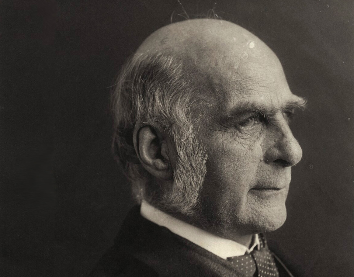
1822–1911

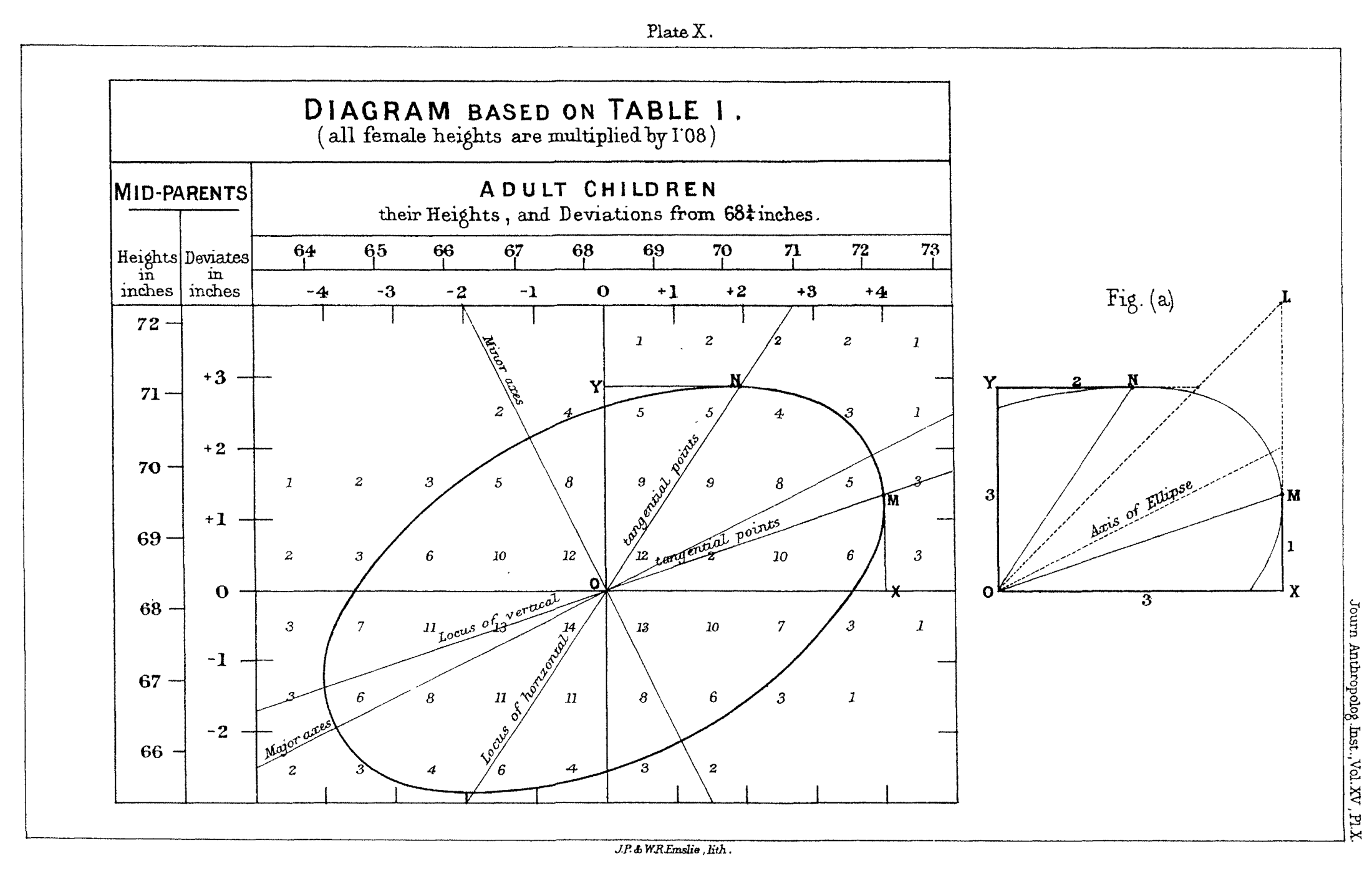
Darwin's half-cousin and a Victorian polymath with interests in heredity, meteorology and statistics. He measured parents' and children's heights, entered the frequencies in a grid and found that the contours formed ellipses.

The shape of the ellipse became his measure of association: a narrow ellipse around a line indicates a strong linear association when the axis scales are fixed. This was correlation, almost a decade before Pearson formalised r (1895–96).

Historical background

Galton's ellipse

Galton 1886, Plate X: ellipse diagram of parents' and children's heights — Figure 2. Plate X from *Regression towards Mediocrity in Hereditary Stature* (1886).

Galton's original diagram from 1886. The printed figures are his approximate interpolated values from a smoothed frequency surface, not raw counts for each cell (original paper, p. 263). The colour layer is a smoothed teaching overlay based on the printed values. The grid includes the confirmed overprinted values 13 and 2; in this display, the isolated dip at 2 has been smoothed using its four neighbours. This is not an exact reconstruction of the original surface. Blank cells remain missing and are not treated as observed zeroes. The tilted ellipse shows correlation: a narrow shape around a line indicates a strong linear association at fixed axis scales. Steepness alone does not tell us how strong the association is. Pearson formalised this as r almost a decade later (1895–96). Regression to the mean: the children's heights regress towards the mean. The ‘locus of horizontal tangential points’ is the regression line.

Correlation

What is r?

Figure 3. r describes the shape of the cloud, not a line through it

Regression

Why is it called regression?

Figure 4. Regression to the mean in two repeated measurements.

Link this back to Galton: regression to the mean is not a force pulling individuals towards an average. The 100 fixed simulated pairs come from fig1.html. Each complete measurement series is standardised separately to a mean of zero and a sample SD of one. All pairs are retained and r is about 0.50. Select the highest fifth, or 20 per cent, using the first measurement alone. This is a simple illustrative selection rule, not a clinical threshold or a condition required for regression to the mean. Assume a stable situation, with no intervention or general change between measurements. The plot is square and both axes use the same standardised scale, so the identity line is at 45 degrees. The figure's own arrows move forwards and backwards through its steps. The arrows in the control bar move straight to another slide. The first click shows the reference lines. Explain aloud that r is about 0.50 and that the identity line is y=x. Two small open triangles, just below the x-axis and to the left of the y-axis, mark the overall means. The second click selects the highest 20 per cent: their opacity stays the same while the other points fade. The third click draws a red dashed vertical line from the x-axis at the selected group's first mean to the top of the plot. The fourth draws a red dashed horizontal line from the y-axis at the same people's second mean to the right edge. A matching open red triangle appears on each axis with its mean line. There are no labels in the margins. In this group, the mean falls from about 1.43 to 0.80 standardised units; 15 of 20 have a lower second value. Individual values need not all fall. The fifth click emphasises the overall means, fades the identity line and draws two red pen strokes just outside the axes. The lower stroke marks the distance from the group's first mean to the overall mean; the left stroke marks the distance from its second mean to the overall mean. The distances, about 1.43 and 0.80, can be compared directly because the axes use the same scale. The point is that the group's mean is closer to the overall mean on retesting. No fitted regression line is shown. The sixth click resets the plot: the red lines and strokes disappear, the identity line returns and all points become opaque. The seventh click selects only the lowest 20 per cent on the first measurement. The eighth shows their first mean with a blue vertical line. The ninth shows the same people's second mean with a blue horizontal line. The tenth draws the corresponding blue distance marks along the axes. Matching blue triangles appear on the axes with the mean lines. Here the mean rises from about −1.35 to −0.54 standardised units; 18 of 20 have a higher second value. The distance to the overall mean therefore decreases from the lower end too. These are the same 100 pairs on the same scale. Selection never uses the second measurement and no point moves. Keep two questions separate. In method comparison, Deming can estimate the underlying relationship when both methods have measurement error. An OLS prediction of the observed second value given the observed first value has a different purpose; it need not estimate the error-free relationship. For a linear conditional-mean relationship with equal SDs, the predictive line has slope r. With equal SDs and an assumed λ=1, Deming would give the identity line here. Replacing OLS with Deming would therefore not explain the retested group's mean. Show the phenomenon through the observed group means without bringing model choice into it. A change after an intervention is not sufficient evidence of a causal effect. The next slide asks a different question: how restricting the measurement range affects r. No real patient data or treatment results are shown. Source for the distinction between a functional relationship and conditional means: Martin Bland, Regression towards the mean, University of York (2004), sections What is regression towards the mean? and Comparison of two methods of measurement. https://www-users.york.ac.uk/~mb55/talks/regmean.htm

Correlation

Restricting the measurement range

Figure 5. Correlation depends on the measurement range we examine.

Agreement

Correlation ≠ agreement

Figure 6. High correlation does not mean that two methods give the same results.

Method performance

What do we need to know?

Loading the measurement data…

Relationship and bias

Deming

Assumed λ = 0.3, constant SD

Differences and dispersion

Mean differenceLoA

Normal approximation, stable dispersion within 0–50

Figure 7c. The same pairs, with estimated bias and individual differences.

Bias at relevant levels

Estimate with 95% CI

Reference level	Bias (95% CI)

Illustrative levels, arbitrary units.

Imprecision from replicates

SD or CV at relevant levels, within and between days.

LoA do not replace a precision study.

A point cloud and r are not enough to assess bias, imprecision or clinical usefulness. Start with the intended use, the relevant patient population, the specimen type and a measurement range that covers medical decision levels. Report estimated bias with confidence intervals at those levels, rather than regression coefficients alone. Regression and the difference plot complement each other. The difference plot shows individual differences and can reveal bias that changes with concentration, varying dispersion and outliers. LoA describe the dispersion of differences between two methods. They can include measurement error from both methods and sample-specific effects; they are not a separate precision study of the new method. Investigate SD or CV using replicates at relevant levels, within and between days. Compare the results with acceptance criteria set before the study. Which differences are acceptable depends on the clinical question. Method comparison alone does not establish clinical suitability. The figures use exactly the same 78 synthetic pairs as the advertisement; 48 have reference values of 0–50. The values 10, 25 and 50 are illustrative levels, not actual medical decision thresholds. Deming is fitted to the pairs with an assumed λ = variance of reference-method measurement error / variance of Super Method measurement error = 0.3, and constant SD. λ is an illustrative analysis assumption, not an estimate from the pairs. The original generator added noise only to y; this is a reporting example under a different assumption, not a validation of Deming against known truth. In practice, precision needs evidence from replicates or a credible precision profile. Weighted Deming may be needed when SD varies. Bias estimates come from regression over 0–200, with 95% CIs from 5,000 paired bootstrap resamples. Fitted regression: y = 1.019x + 1.81; 95% CI for the intercept −0.35 to 3.81. Mean difference within 0–50: 1.92, 95% CI 0.20 to 3.68. LoA −10.32 to 14.15; 95% CI for the lower limit −13.57 to −6.73 and for the upper limit 10.78 to 17.40. These LoA use a normal approximation and assume stable dispersion within 0–50. The teaching data contain neither a separate imprecision study nor actual clinical acceptance criteria. The known generating slope of 1.05 falls just outside the estimated 95% interval of 0.995 to 1.048. A single interval need not include the generating parameter; this alone does not establish a calculation error. Keep the generating truth, the analysis error model and the fitted line separate. Sources: CLSI EP09c, 3rd edition, 2018, sections on bias at clinical decision levels, difference plots and CIs; its scope points readers to EP05/EP15 for separate precision studies. https://clsi.org/shop/standards/ep09/ and https://clsi.org/shop/standards/ep15/.

Agreement

Does a mean bias of 16 tell us enough?

Figure 8. The difference between the methods increases with the measured value.

Regression models

OLS: the default we take for granted

Figure 9. OLS minimises the sum of squared vertical residuals.

Regression models

Deming: measurement error in both methods

Figure 10. Deming accounts for measurement error in both methods. Schematic residuals.

Deming minimises a variance-weighted criterion for distances along both axes, accounting for measurement error in both methods. The readout is labelled Sum of squares in both the OLS and Deming figures. OLS sums the squared vertical residuals. Deming shows the weighted sum of squares Q_λ = Σ[(x−x̂)² + λ(y−ŷ)²]. The fit and sum of squares are calculated in measurement units. The red lines are schematic: the display-scale correction is used only for drawing, so that λ = 1 looks perpendicular even in the wide plot. For drawing, λ is multiplied by (display scale y / display scale x)²; this does not change the model's error ratio. Do not use the drawn line lengths to calculate the sum of squares. The value appears only when the line is visible and is calculated from the statistical projections in measurement coordinates. For a given λ, it has the same minimum as the usual Deming criterion. Compare lines at the same λ; do not compare sums across different λ values to choose an error ratio. λ is the ratio of the methods' measurement-error variances, λ = σ²(reference)/σ²(test), following the convention in Linnet (Clin Chem 1998) and the R package mcr. High λ means more measurement error in the reference method, and the residuals tilt towards the horizontal. Low λ means more measurement error in the test method, and the residuals approach OLS. λ = 1 (orthogonal regression) is a common assumption when imprecision data are unavailable, but it assumes equal measurement error. Base λ on imprecision data, not on scatter around the regression line. Duplicates in the comparison study itself are the best source: within-sample replicates are independent of the x–y relationship and give λ directly (Linnet, Clin Chem 1998; CLSI EP09c 6.2.2). Without replicates, use imprecision from EP05 studies or QC data. If neither is available, set λ = 1 and examine sensitivity to other values (EP09c 6.2.2). Estimating λ from residual scatter in single measurements is circular. Show how the residual angle changes with λ. CLSI EP09c (3rd edition, 2018) recommends Deming as the default, with the variant determined by the error structure: constant-SD Deming for constant SD across the measurement range (6.2.1), and weighted constant-CV Deming for constant CV (6.2.2). Passing–Bablok is listed as an option for constant CV and as the first choice for unusual or skewed distributions (6.2.4).

Regression models

Passing–Bablok: the robust alternative

Figure 11. Passing–Bablok uses ranked pairwise slopes.

Non-parametric: based on ranked pairwise slopes. Classical Passing–Bablok uses a shifted median and special rules for certain slopes; the animation illustrates the principle. It is robust to outliers and does not require a normal distribution, but it is not assumption-free. A confidence interval that includes slope 1 or intercept 0 does not show that the methods are interchangeable. Assess bias and dispersion against clinical acceptance limits set in advance. Passing–Bablok implicitly assumes that SD(test)/SD(reference) equals the slope β (variance ratio β²): errors are proportional to each method's scale (EP09c app. I; Baumdicker and Hölker, Stat Probab Lett 2020, remark 2.5). If β is expected to be close to 1, this assumes roughly equal measurement-error SDs. At similar levels, that corresponds to roughly equal CVs. A slope near 1 is therefore not enough: substantially different imprecision can still be a problem. The method's CUSUM linearity test uses the signs of deviations from the line, ordered along the line. PB does not specify a normal-based residual model. Its parameter estimates still have uncertainty: standard errors and confidence intervals can, for example, be estimated by bootstrap. Confidence intervals for the slope and intercept are calculated analytically (EP09c app. I). Confidence intervals for bias at a decision level require bootstrap (EP09c app. K2); jackknife gives unrealistically narrow intervals because a single point rarely moves the median. PB can be a robust alternative for outliers or unusual distributions, provided linearity and the error relationship are reasonable. Heteroscedasticity alone does not determine the model choice; with constant CV and known imprecision, weighted Deming is a natural choice. PB is not generally better or worse than Deming.

Regression models

What happens when we add outliers?

Figure 12. The same pairs and the same outliers for all three models.

Separate robustness to isolated outliers from modelling analytical imprecision. Here, 60 fixed simulated pairs lie around the true relationship y=x, with independent normally distributed measurement error of SD 4 in both methods. Deming therefore uses λ=1. This is the stated generating error ratio, not a ratio estimated from the point cloud. The seed is fixed at 20261015 and is independent of the lecture's other examples. The four round buttons each switch a predefined outlier on or off: (76,132), (83,147), (69,138), (91,129). First add them in order 1–4, then try switching individual points off or combining them. The numbers beside the points match the buttons. The red points have large positive y deviations. The original points do not move, all three models are refitted to exactly the same 60–64 pairs, and the axis scales stay fixed. Here the slopes change from about 0.96 to 1.14 for OLS, from 1.00 to 1.36 for Deming, and from 0.99 to 1.05 for classical Passing–Bablok. Look at the changed intercepts too. PB is affected least by these particular added points. This is a deliberate illustration of contamination, not a comparative simulation study or evidence that PB is always best. The number and position of outliers, their leverage and the rest of the error structure matter; PB can also be affected. Ordinary Deming and OLS have quadratic criteria and are not robust regression methods. Accounting for measurement error on both axes does not automatically make Deming robust to outliers. Investigate outliers; do not delete them simply because the line looks better. Source: NIST Dataplot, Passing Bablok Fit, method-comparison variant, https://www.itl.nist.gov/div898/software/dataplot/refman1/auxillar/pb_fit.htm. The next example, Regression dilution, asks a different question. In that example, Deming's λ follows the known simulated error ratio SD(x error)²/SD(y error)². λ=1 is not generally correct when imprecision is unknown. Linnet, Clin Chem 1998;44:1024–31, https://pubmed.ncbi.nlm.nih.gov/9590376/.

Regression models

Regression dilution

Figure 13. Measurement error in x attenuates the OLS slope.

Regression models

Model convergence

Figure 14. OLS, Deming and Passing–Bablok with adjustable correlation.

Demonstrations 1 and 2. An r slider from 0.80 to 0.99, with three fitted lines. The models often converge when random measurement error is small relative to the clinically relevant measurement interval. Raise r to 0.99 to reveal the question mark. Click it to zoom in on the twenty central observations in a narrower x interval. Once the animation finishes, all three models are fitted to those pairs and the correlation in the selected range appears below the plot. The slider still reports r for the whole cloud. The return arrow restores the full cloud. Do not say that model choice no longer matters at r > 0.99. That would undermine the point about range restriction: r depends on the sample range, not just the method's precision. Say instead that the models converge at low measurement error, but the error structure determines the choice, not the r value.

Regression

What regression tells us

Slope ≠ 1: proportional bias

Intercept ≠ 0: constant bias

R² = 1 − SS_res / SS_tot

SS_res: the sum of squared vertical distances from the points to the regression line — the variation that remains.

SS_tot: the sum of squared deviations of the y values from their mean — the total variation.

R² = 0.90 means that 10% of the total sum of squares remains as residual variation.

r measures linear association. R² = r² holds for simple OLS with an intercept.

r tells us very little about agreement when r > 0.98. It still has a supporting role: EP09c app. G uses r ≥ 0.975 to check that the x range is wide enough for OLS to be defensible, not as a measure of agreement. Recalibrating one method against another requires the equation. R² is the coefficient of determination: 1 − (residual sum of squares / total sum of squares). SS_tot = Σ(y_i − ȳ)² is the total sum of squares about the mean. SS_res = Σ(y_i − ŷ_i)² is the residual sum of squares about the fitted line. These are sums of squares, not variances in themselves. Compare the fitted line with the simple prediction that every y value equals the mean. If SS_tot = 100 and SS_res = 10, R² = 0.90. The coefficient of determination describes fit, not a causal explanation or agreement between methods. R² tells us how much of the variation in y the model explains. Pearson's r measures linear association between x and y; it is a descriptive measure independent of which model is fitted. R² = r² holds only for OLS, where minimising vertical residuals makes correlation and the coefficient of determination coincide algebraically. The same ratio can be calculated for Deming and Passing–Bablok, but it does not have the OLS model's variance decomposition and should not be used as a general measure of model suitability. Do not go further into R² here. The point is that r and R² are different measures answering different questions.

Visual inspection

Can you see a difference?

Figure 15. Anscombe's quartet: four different patterns with the same summary statistics.

Visual inspection

Regression models have no eyes

Figure 16. Different point patterns with the same summary statistics.

Thinking about models

Ptolemy's geocentric model with epicycles — Figure 17. A geocentric model with epicycles.

All models are geocentric

The same statistical measures can describe very different point clouds.

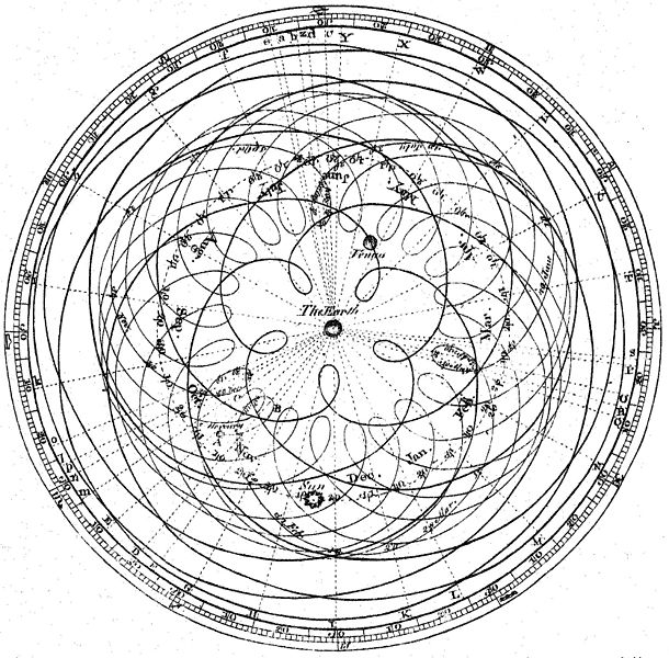
Ptolemy's epicycles predicted planetary positions with great precision. But the model put the Earth at the centre.

All regression models are geocentric, but not equally geocentric. Assumptions about the error structure determine the slope we get.

Visual inspection

A linear relationship?

Figure 18a. Two biochemical markers in an illustrative dataset.

The figure's own arrows move through two examples and their reveals: two clouds in black; the pooled regression line; the line removed; the populations coloured; Berkeley totals; departments; then five steps in the constructed regression example. The presentation's usual navigation arrows go straight to the previous or next slide. This reconstructs a plot the lecturer remembers from specialist training. The markers, values and group sizes are illustrative. These are not original data and do not reproduce an identified study. There is a large, roughly round cloud and a smaller cloud to its right and slightly higher, with sparse, evenly distributed points between them. The cloud cores are generated with independent x and y deviations. The points between them also have fixed membership of one of the two populations. Association in the pooled data is driven mainly by the clouds' different positions. Ask what a single line actually summarises and whether it describes variation within each population. Such a plot alone establishes neither which populations exist nor their biological explanation. Initially, all points are black. The next figure step draws a pooled Deming line with λ = 1 through all 237 observations, including the 22 intermediate points. The line is fitted in data coordinates, not display pixels. This is a deliberately naive fit to a mixture of populations. Equal error variance on the axes is an illustrative assumption, not an estimated precision profile. The next step fades the line without colouring the points yet. Then all 237 observations are coloured: 175 blue and 62 muted red, with the same opacity. Every point belongs to a population. The 22 intermediate points keep their original coordinates. Their fixed membership is defined when the teaching example is built, using each cloud's relative density from the predefined centres (32,26) and (79,40), SDs 8.5 and 5.2, and sizes 160 and 55. The rule does not use the regression line or search for desired correlations. Some points therefore lie visibly far from their population's core. These are constructed memberships, not an analysis identifying real patient groups. All point positions, scales and memberships remain fixed; clicking neither selects points nor simulates new ones. With all observations included, r is about 0.078 in the blue population and 0.097 in the red: weak in both. The pooled positive association is driven by different group levels and does not imply a linear relationship within the populations. Colours show the example data file's fixed group memberships; colouring does not perform a new classification. A real analysis requires knowledge of the populations and sampling. Example 2 uses actual Berkeley data from autumn 1973, for the six largest departments A–F: 4,526 applicants, not all 12,763 applications to the university. First show the overall admission rates: 1,198 of 2,691 men (44.5%) and 557 of 1,835 women (30.4%). The next figure step shows the six departments on the same axes, while the total points, values and summary row are hidden. Total points have black outlines and transparent fills, with a dashed black line joining the circle edges. The line connects two proportions; it is not a regression model. Department points are paired with dashed lines in matching colours, running from circle edge to circle edge. The points have solid coloured outlines and translucent fills. Letter labels within the plot are hidden. There are no subject names or other notes in the left margin. The departments are anonymised as A–F in the source data. Here x is sex, not a continuous measurement variable; y is the admission rate as a percentage. No regression is fitted. Circle area is proportional to the number of applicants, with the same area scale for totals and departments. A: men 512/825, women 89/108. B: men 353/560, women 17/25. C: men 120/325, women 202/593. D: men 138/417, women 131/375. E: men 53/191, women 94/393. F: men 22/373, women 24/341. Women have higher admission rates in four of the six departments: A, B, D and F. Do not say all six. Among men, 51.5% apply to A/B; among women, 7.2%. Applicants are distributed differently across departments with different admission rates, so the overall result does not describe the comparison within departments. The figure estimates no adjusted causal effect and supports no general conclusion about fairness. Source: R's UCBAdmissions, https://stat.ethz.ch/R-manual/R-devel/library/datasets/html/UCBAdmissions.html. Source data: https://raw.githubusercontent.com/wch/r-source/trunk/src/library/datasets/data/UCBAdmissions.R. Bickel PJ, Hammel EA, O'Connell JW. Sex Bias in Graduate Admissions: Data from Berkeley. Science 1975;187:398–404. doi:10.1126/science.187.4175.398. The final figure in the Berkeley sequence is a separate constructed example with continuous variables. It is not a replot of Berkeley data or a ‘degree of being female’. There are six groups of 40 observations each, with fixed seed 20261019. Group centres run from (24,72) to (76,28), in steps of (10.4, −8.8). The groups' x ranges overlap. Within each group, a latent x coordinate varies uniformly from −9 to 9. The slopes are 0.45, 1.2, 0.75, 1.55, 0.6 and 1.05. Independent normally distributed measurement errors in X and Y both have SD 1.8. No extra noise points have been added. All models are Deming with λ = 1: the same error model within groups and in the deliberately naive pooled fit. Every group has a positive association, while the pooled data have a negative association. The five figure steps are: all points black with no model; draw the negative pooled line; fade that line; colour the subgroups; draw the six positive within-group lines. The pooled and within-group models are never shown together. Points and scales never move between steps. All views omit axis titles, tick values and group letters. Within-group and between-group comparisons answer different questions. No causal effect is estimated. Do not attribute this figure to Bickel or interpret it as individual Berkeley data.

Error structure

Constant SD or constant CV?

Constant SD

Roughly the same absolute dispersion.

Constant CV

Dispersion increases with concentration.

Figure 19. Illustrative residuals around a correctly specified linear relationship: the same noise pattern on different scales.

A closer look: error structure

Three approaches, different assumptions

Weighted Deming

Models measurement error in both methods. With constant CV, it uses concentration-dependent variances.

Imprecision data determine the error model. High concentrations should not dominate simply because their absolute variance is larger.

Log scale

Can stabilise proportional dispersion for positive values, but also changes the relationship being modelled.

log y = α + β log x
y = e^αx^β

Passing–Bablok

Uses ranked pairwise slopes and is less sensitive to isolated outliers. Does not use measured imprecision data.

When the methods are expected to give the same values, roughly equal measurement-error SDs are assumed.

an optionwith outliers

Weighted Deming: with constant CV, variance is proportional to concentration squared; the weights incorporate both methods' imprecision and estimated levels. Log–log regression gives a power relationship after back-transformation, not generally y=a+bx. That relationship describes the back-transformed fitted log level; predicting the mean on the original scale may require further allowance for the error model. Passing–Bablok uses a shifted median and special rules for pairwise slopes. This detailed slide can be skipped during the talk. CLSI EP09c, 3rd edition, 2018: original PDF in Zotero, parent item 7W9U3GEN, attachment PIC3B5C7. Sections read in full for the source lecture: 6.2.1–6.2.4, appendices B and J. Section 6.2.1 gives constant-SD Deming as the default. Section 6.2.2 gives constant-CV Deming as the default and warns against comparing a transformed slope with acceptance criteria on the original scale. Sections 6.2.3–6.2.4 describe Passing–Bablok for mixed variability and unusual results. With known precision profiles, section 6.2.3 and appendix J describe profile-weighted Deming as an option. PDF pages 25–27, 34–35 and 56–57 (63-page eCLIPSE printout). This summarises CLSI; it does not imply that Passing–Bablok has no assumptions of its own. NIST Passing Bablok Fit.

Weighting

What do we actually do when we ‘weight’ a regression model?

The CV is the same, but SD increases with the level.

Ten times the SD means one hundredth of the weight.

Figure 20. The same relative deviation: different contributions before weighting, equal afterwards. Schematic example in arbitrary units.

This is a schematic residual plot, not a scatter plot of method values. The grey band shows ±1 expected SD, not a confidence interval or a clinical acceptance range. The other points form a fixed illustrative residual distribution; the SD profile is specified in advance. The diagonally hatched square areas use the same scale (64 SVG area units per unit of contribution) before and after weighting. The displayed line stays fixed: weighting changes the contributions to the criterion, not the observed data. During fitting, the criterion is evaluated for different candidate lines. This is a concrete but illustrative example with a constant CV of five per cent, in arbitrary units. The reference levels are 20 and 200. Assume a correctly specified linear relationship and expected SDs around the line of 1 and 10, respectively. The observed deviations are 2 and 20: both lie two SDs from the line. Without variance weighting, their contributions to the sum of squared residuals are 4 and 400. With weights proportional to inverse error variance, the contributions are 4 and 4. The high-level point has one hundredth of the low-level point's weight, not the same weight. It is the weighted contributions that happen to be equal in this example. This does not give the points identical influence on the slope or equal clinical importance: x position, the other data and clinical acceptance criteria also matter. The weights come from expected imprecision, not from how well a particular observed point fits the line. On one click, the large square shrinks to one tenth of its width and height, hence one hundredth of its area. The small square is unchanged. At the same time, w_i=1/sigma_i² and Q=sum_i w_i e_i² appear. Q is the criterion being minimised, not an estimate of clinical importance. Use e for the residual to avoid confusing it with the correlation coefficient r. WLS can be mentioned aloud: it stands for weighted least squares. Mathematically, divide each residual by its expected SD, square it and add the results. This is equivalent to multiplying each squared residual by the weight 1/SD², or inverse variance. Calculate these contributions for each candidate line and choose the line giving the smallest sum. Here SD describes dispersion of the y error around the correct relationship at a given x, not the standard error of mean bias. The simple numerical example assumes negligible measurement error in the reference and a known SD profile. Otherwise, weights need evidence from replicates or a credible precision profile; they are not set to the inverse of a single observed residual. At constant CV, SD grows with the level and variance weights decrease with the square of the estimated level. Do not routinely use 1/y² from each noisy observed value. Weighting does not correct attenuation from measurement error in x. With measurement error in both methods, a model such as weighted Deming is needed: both x and y deviations are compared with their respective measurement-error variances. Variance weighting is not automatically robust to outliers. Source: NIST/SEMATECH e-Handbook, 4.1.4.3, 4.4.3.2 and 4.4.5.2; https://www.itl.nist.gov/div898/handbook/pmd/section1/pmd143.htm and https://www.itl.nist.gov/div898/handbook/pmd/section4/pmd452.htm.

Summary

Why model choice matters

r measures association, not agreement, bias or interchangeability.
OLS does not account for measurement error in x. Classical independent measurement error in x attenuates the slope.
Deming models error in both axes, with an error ratio and weighting that need to reflect the methods' imprecision.
Passing–Bablok is less sensitive to isolated outliers, but does not use measured imprecision data. When the methods are expected to give the same values, a central assumption is roughly equal measurement-error SDs.
When measurement error is small relative to the measurement range, the models converge. The error structure determines the choice, not the r value.

Back in the laboratory

How we assess the new method

Plot the data. Relationships, differences, outliers and measurement range.
Examine the error structure. SD, CV and imprecision in both methods.
Choose a model. Check linearity and the relevant assumptions.
Estimate bias and uncertainty at clinically relevant levels.
Compare with predefined requirements. Is the evidence sufficient?

Set the acceptance criteria before the study.

References

CLSI EP09c, 3rd ed. 2018. Measurement Procedure Comparison and Bias Estimation Using Patient Samples. Ch. 6.2 (regression choice), app. B (weighted Deming), app. G (r and the x range), app. I (Passing–Bablok), app. K (CIs for bias).
Linnet K. Performance of Deming regression analysis in case of misspecified analytical error ratio. Clin Chem 1998;44:1024–31.
Linnet K. Necessary sample size for method comparison studies based on regression analysis. Clin Chem 1999;45:882–94.
Stöckl D, Dewitte K, Thienpont LM. Validity of linear regression in method comparison studies. Clin Chem 1998;44:2340–6.
Passing H, Bablok W. J Clin Chem Clin Biochem 1983;21:709–20 (Part I) and 1984;22:431–45 (Part II).
Baumdicker F, Hölker U. Stat Probab Lett 2020;164:108801.
Galton F. Regression towards mediocrity in hereditary stature. J Anthropol Inst 1886;15:246–63.
Anscombe FJ. Am Stat 1973;27:17–21.
Matejka J, Fitzmaurice G. Same stats, different graphs. CHI 2017.
Bland JM, Altman DG. Measuring agreement in method comparison studies. Stat Methods Med Res 1999;8:135–160.
NIST Dataplot. Passing Bablok Fit.
NIST/SEMATECH e-Handbook. Weighted least squares regression, sections 4.4.3.2 and 4.4.5.2.
CLSI EP05 and EP15. Studies and verification of imprecision.
McElreath R. Statistical Rethinking, 2nd ed. 2020, ch. 4.

‘The task is not so much to see what no one has yet seen, as to think what no one has yet thought about what everyone sees.’

Arthur Schopenhauer, Parerga und Paralipomena (1851)

Filip Landgren

filip.landgren@gmail.com
https://klinkemipedia.se

View this presentation on a computer

The Line and the Cloud

A visual guide to regression modelsin clinical chemistry

Sir Francis Galton

Galton's ellipse

What is r?

Why is it called regression?

Restricting the measurement range

Correlation ≠ agreement

What do we need to know?

Relationship and bias

Differences and dispersion

Bias at relevant levels

Imprecision from replicates

Does a mean bias of 16 tell us enough?

OLS: the default we take for granted

Deming: measurement error in both methods

Passing–Bablok: the robust alternative

What happens when we add outliers?

Regression dilution

Model convergence

What regression tells us

Can you see a difference?

Regression models have no eyes

All models are geocentric

A linear relationship?

Constant SD or constant CV?

Constant SD

Constant CV

Three approaches, different assumptions

Weighted Deming

Log scale

Passing–Bablok

What do we actually do when we ‘weight’ a regression model?

Why model choice matters

How we assess the new method

References

A visual guide to regression models
in clinical chemistry